6. Issues of Statistical Generalization

When maps are used to display statistical information, cartographers take special care to depict as accurately as possible the underlying distribution of data. This is a difficult task because the whole point of displaying the data cartographically is to generalize the data to facilitate the search for spatial patterns. But by generalizing and simplifying the data, the cartographer may just as easily obscure subtle gradations in the underlying distribution. Therefore, in mapping statistical data, the cartographer is always trying to strike a balance between remaining true to the underlying data distribution and generalizing the data sufficiently to reveal intrinsic spatial patterns.

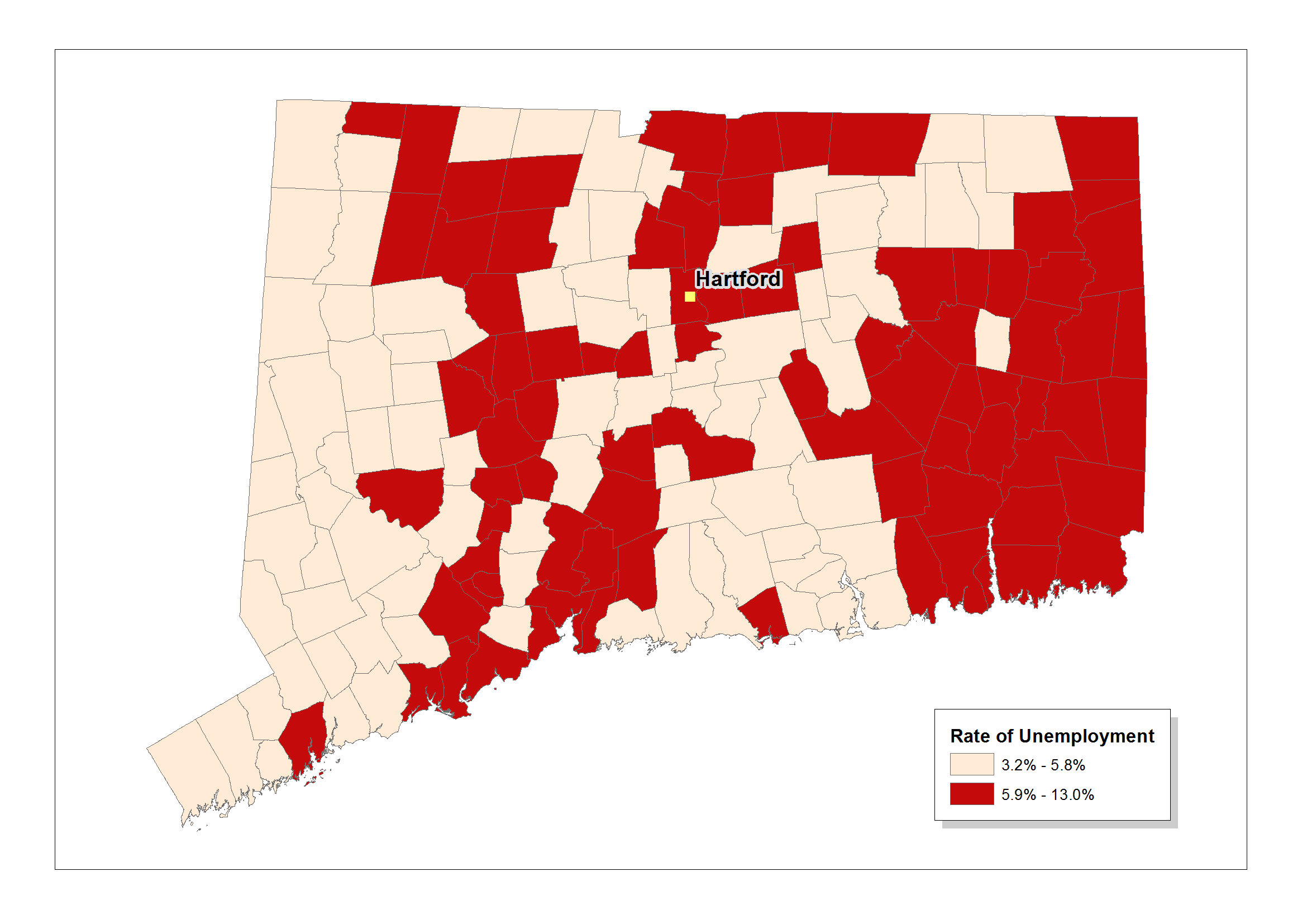
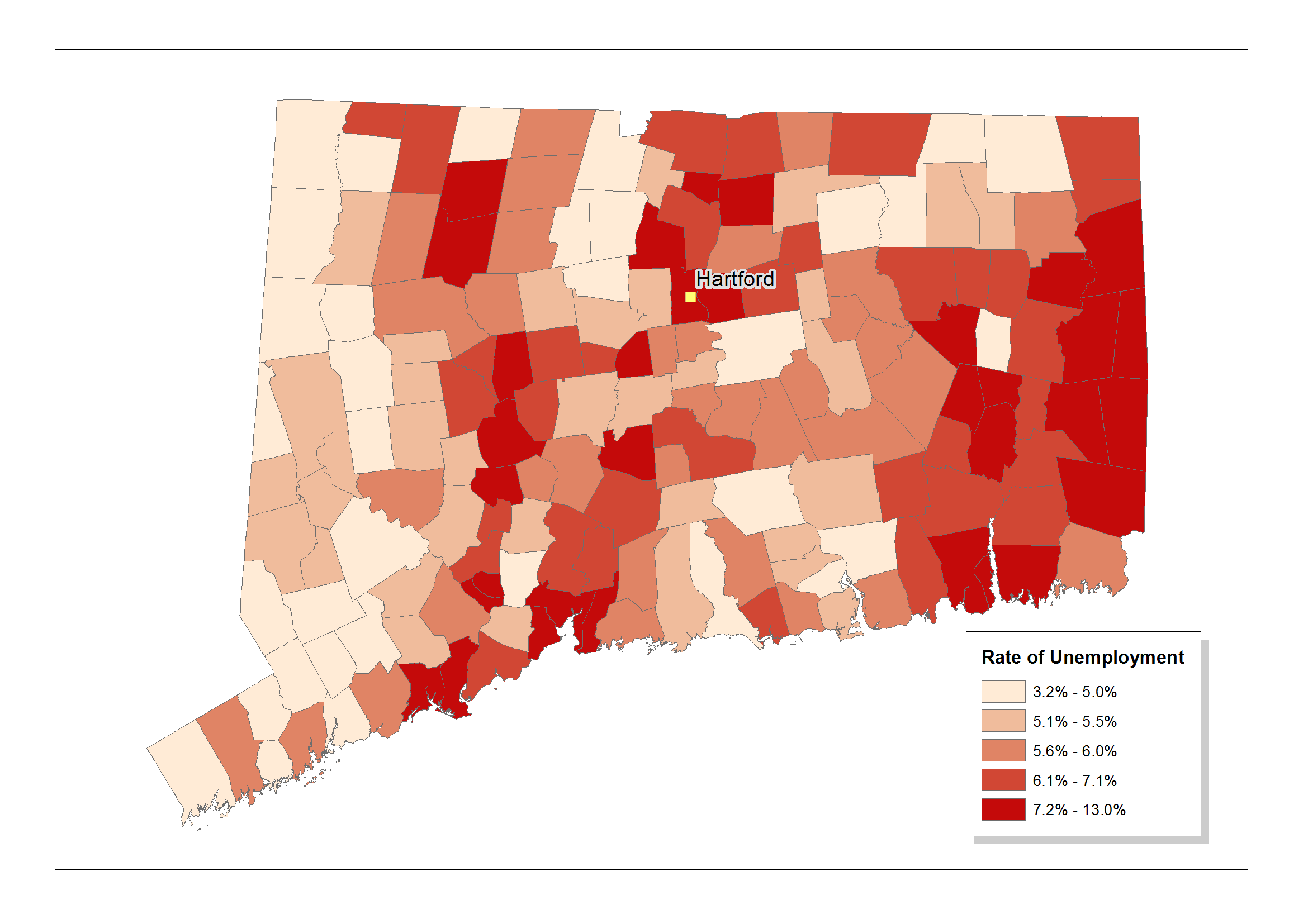
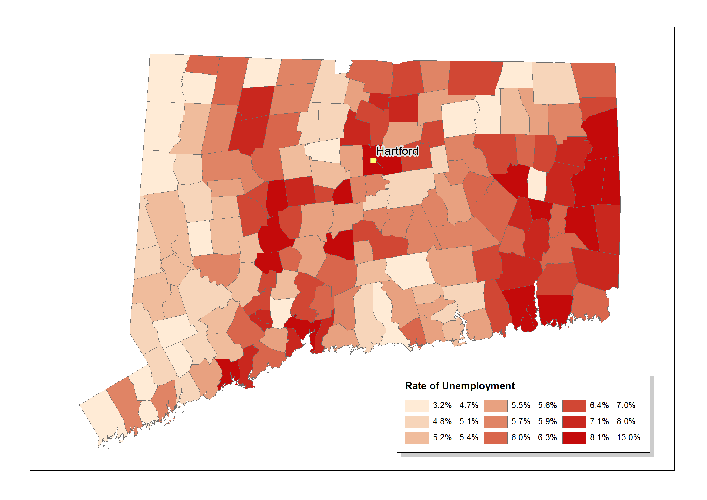
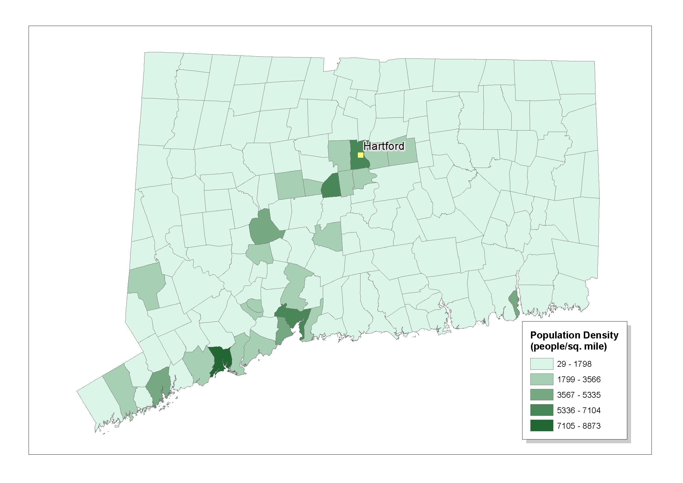
 Although these issues of statistical generalization can be applied to data that is to be symbolized by points, lines, and areas, this discussion will be developed around the mapping of areas in choropleth maps. This is in part because choropleth maps are used so widely, but also because they are difficult to execute effectively. This is because choropleth maps have an inherent weakness - they involve the aggregation of data within areal units that do not correspond exactly with the underlying spatial distribution of data. By focusing on choropleth mapping in the following examples, some of these weaknesses can be revealed and discussed.

To understand the importance of this issue, it is useful to examine a set of maps developed from the same dataset using different numbers of categories and different ranging methods.
A. Comparison of maps using different numbers of categories

 In the example below three maps are divided into quantiles of two, five, and nine categories, respectively.

Unemployment Rates in Connecticut Towns, 2013.
• Map of two categories

• Map of five categories

• Map of nine categories

 If too few categories are used, the map may obscure the contours of the data distribution. Too many categories are just as fruitless and equally unlikely to reveal any existing spatial patterns in the dataset. Indeed, it is difficult for most map readers to distinguish among more than about seven categories. Beyond seven, a map becomes little more than an illustrated table. Most statistical maps will use between three and seven categories.

 B. Comparison of maps using different ranging methods

 These three maps each have five ranges of data, but they were determined using different methods.

• Equal step

• User defined ranges

• Quantile


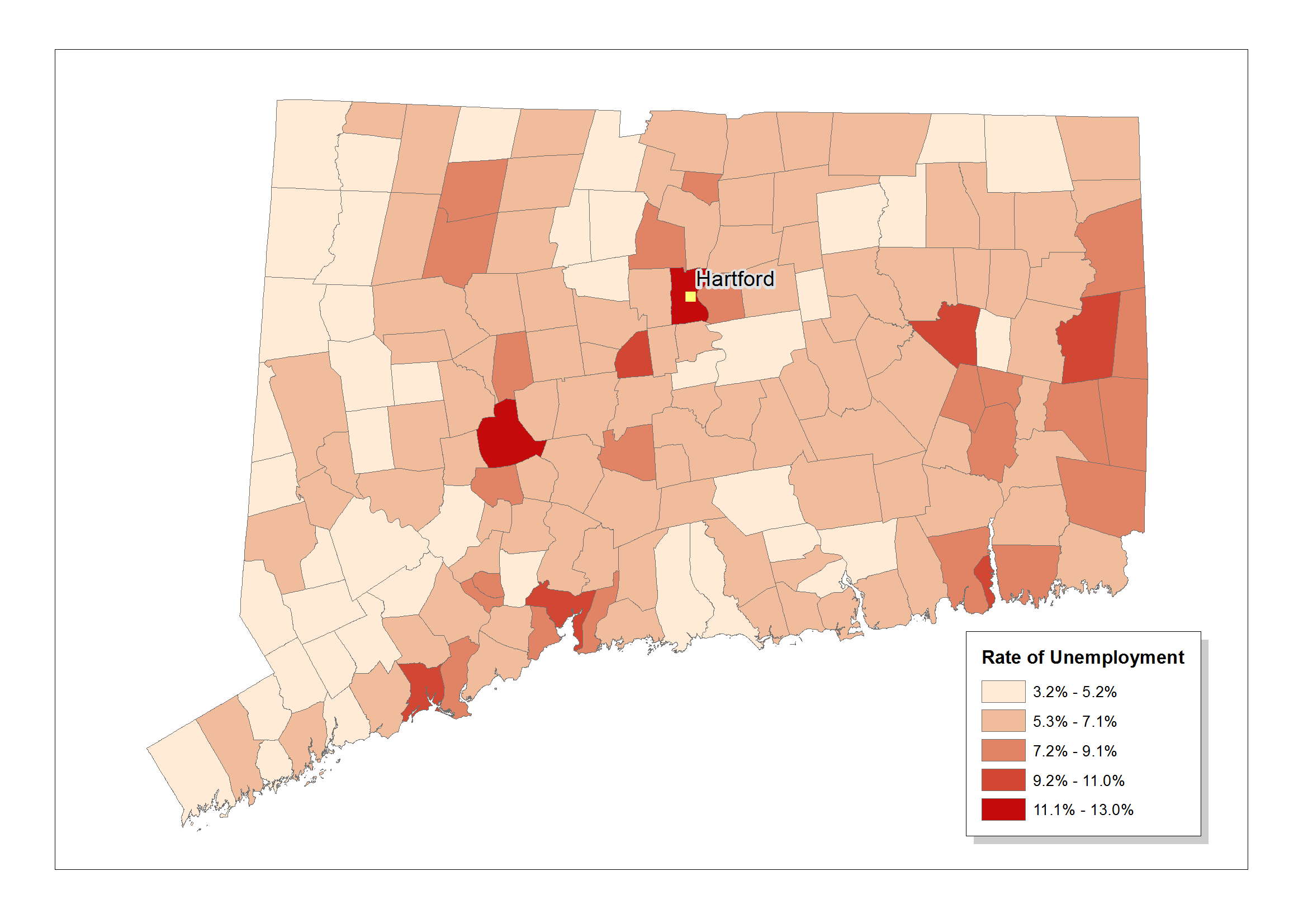
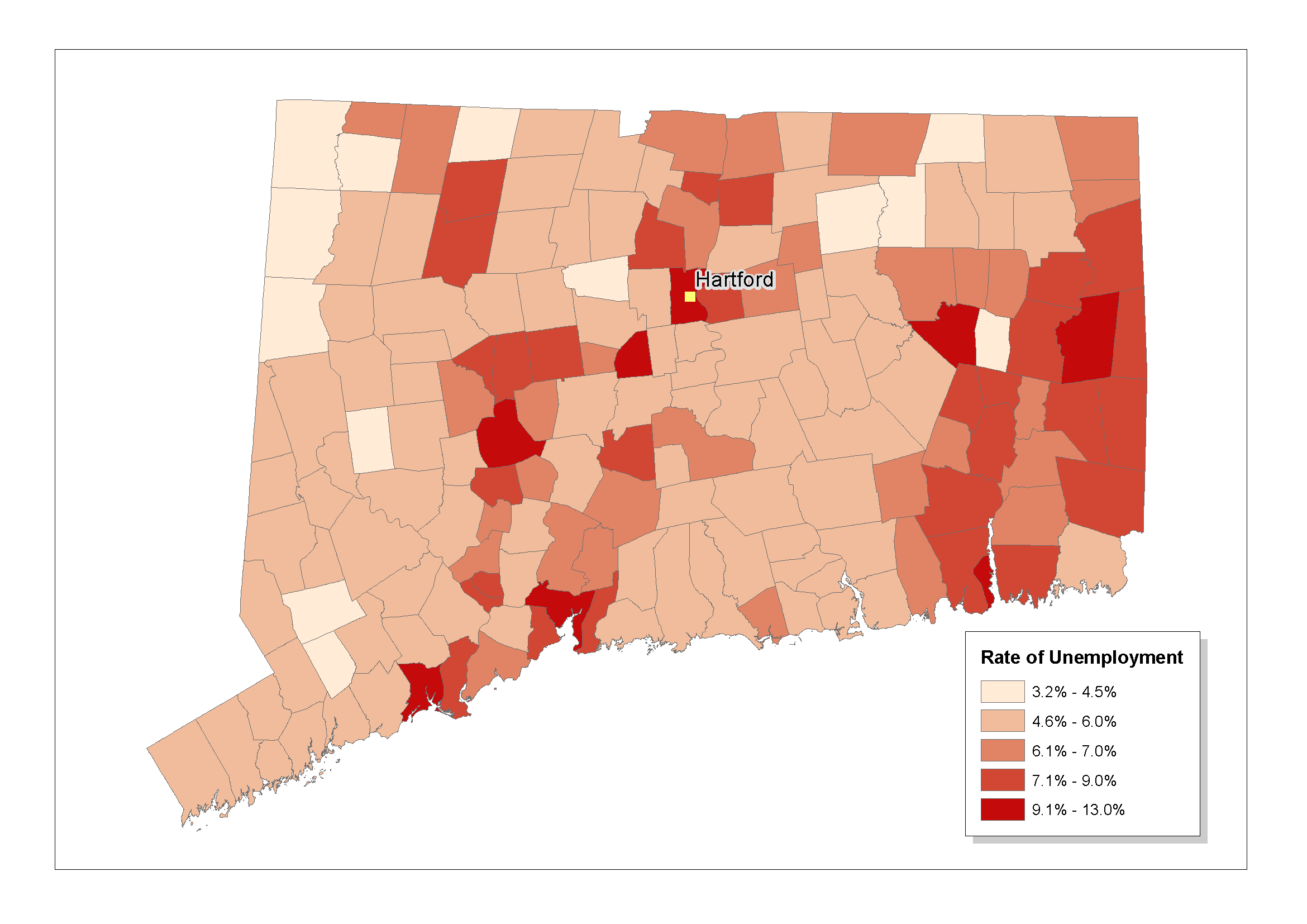
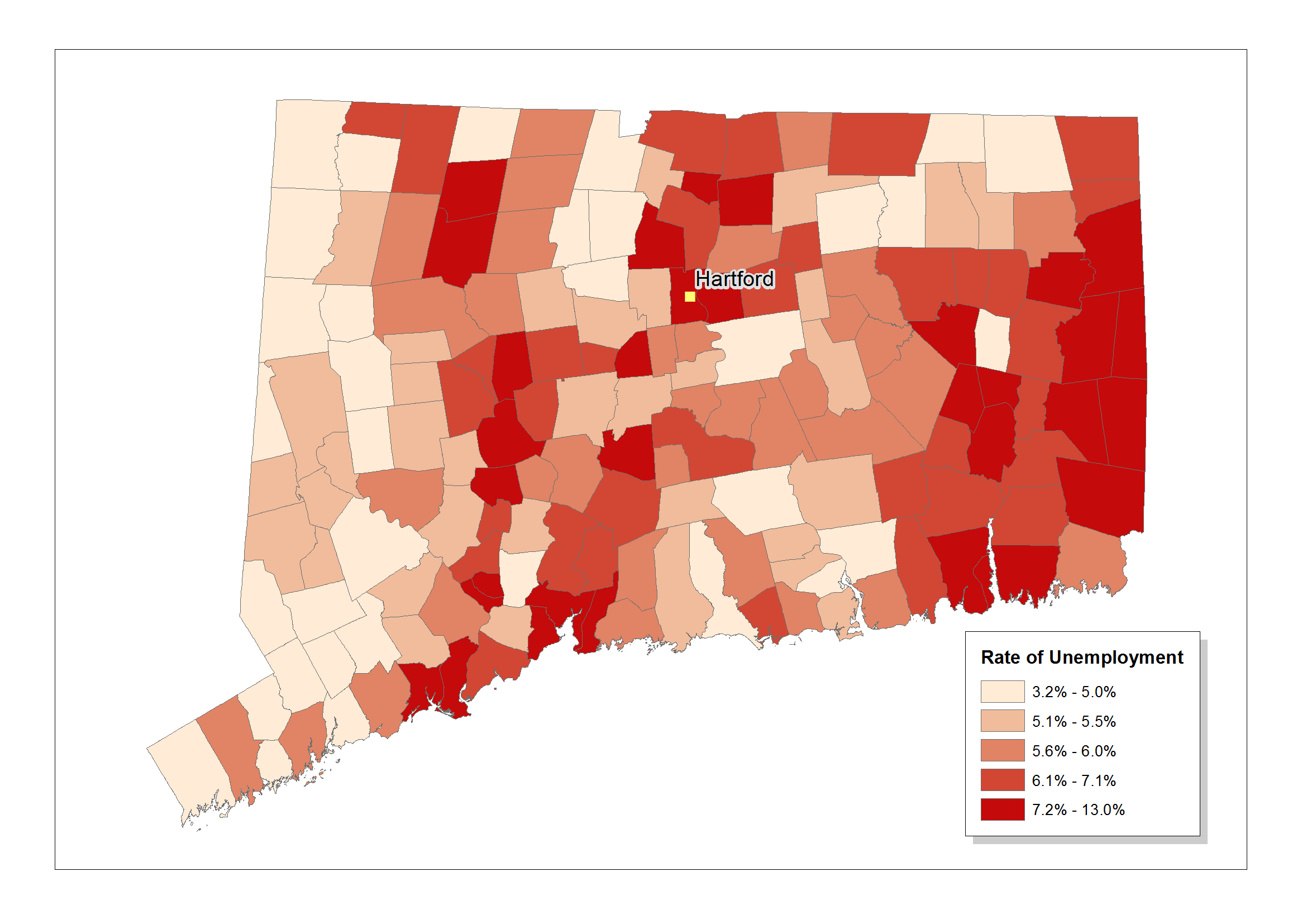
Even though these maps were developed from the same dataset, they seem to convey quite different spatial patterns. Some seem to stress the lowest values in the distribution, others the highest. The point is that cartographers use different ranging methods to generalize different types of data distributions. Each method is suited to a particular "shape" distribution. Therefore, the first step in preparing a choropleth map is to explore the dataset to come to an understanding of its underlying distribution.

6.3 Exploring your data and its "shape"

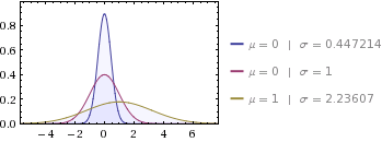
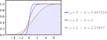
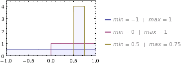
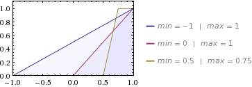
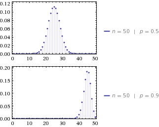
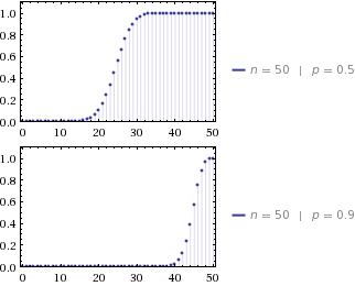
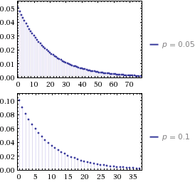
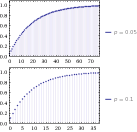
You should get to know the shape of any statistical distribution you plan to map. Plot a scattergram or histogram of the data and employ basic descriptive statistics to explore its distribution. Many automated mapping programs provide options which graph data and will automatically calculate descriptive statistics like mean, mode, median, range, and standard deviation. Take advantage of these options explore your data.

Be aware also that mathematical transformations change the shape of a distribution--implying that the ranging method must change also.

---

Distribution Name and Its Main Parameters	Probability Density Function (PDF)	Cumulative Distribution Function (CDF)

---

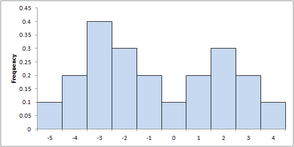
Not all distributions are "well-behaved". Sometimes you can encounter a bimodal (double-peaked) shaped distribution.




6.4 Commonly employed ranging methods for assigning cutpoints

The articles listed below by Michael Coulson (1987), Ian Evans (1977), and George Jenks (1963) provide detailed overviews of the ranging methods commonly employed by cartographers as well as necessary computational algorithms. It is essential that you consult these articles as soon as possible because they cover many more techniques than can be discussed here, and in far greater detail. The following discussion will simply highlight a few of the methods that many computer systems provide as "defaults."

 In generalizing statistical distributions, cartographers use the term "cutpoint" to refer to the boundaries between categories. All the following methods pertain to the calculation or assignment of these cutpoints. Remember, all systems of classification depend upon the use of "exhaustive" and "mutually exclusive" categories. Exhaustive means that the categories classify all values of a given data range--no values within that range are omitted from the classification system. Mutually exclusive means that any given observation can be placed in one and only one category - data categories cannot overlap. Please be sure, if you are using an automated mapping system, that the the system does not assign overlapping cutpoints automatically when it creates the map legend.

A. Equal Steps


This method takes the difference between the low and high values of a distribution and divides this difference into evenly spaced steps. If the 0 and 10 were the low and high values of a distribution and you decided to divide the data into five categories, the cut-points would be: 0, 2, 4, 6, 8, and 10.

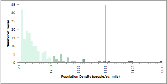
 The method is useful for mapping rectangular (uniform) distributions. It is also useful for exploratory analysis, at times when you wish to develop a "feel" for the characteristics of a data distribution.

B. Quantiles and Percentiles



This method arranges your observations from low to high and places equal numbers of observations in each category. If your data included one hundred observations and you wished to divide the data into five categories (quantiles), the lowest twenty observations would be placed in the first category, the next twenty in the second, and so forth until the highest twenty observations were placed in the last category. The term quartiles is used when the data is divided into four categories, quantiles when five are used, sextiles for six, septiles for seven, and so forth. Note that when data is divided in this way, the cutpoints of the distribution may be arranged at irregular intervals along the span of the distribution.

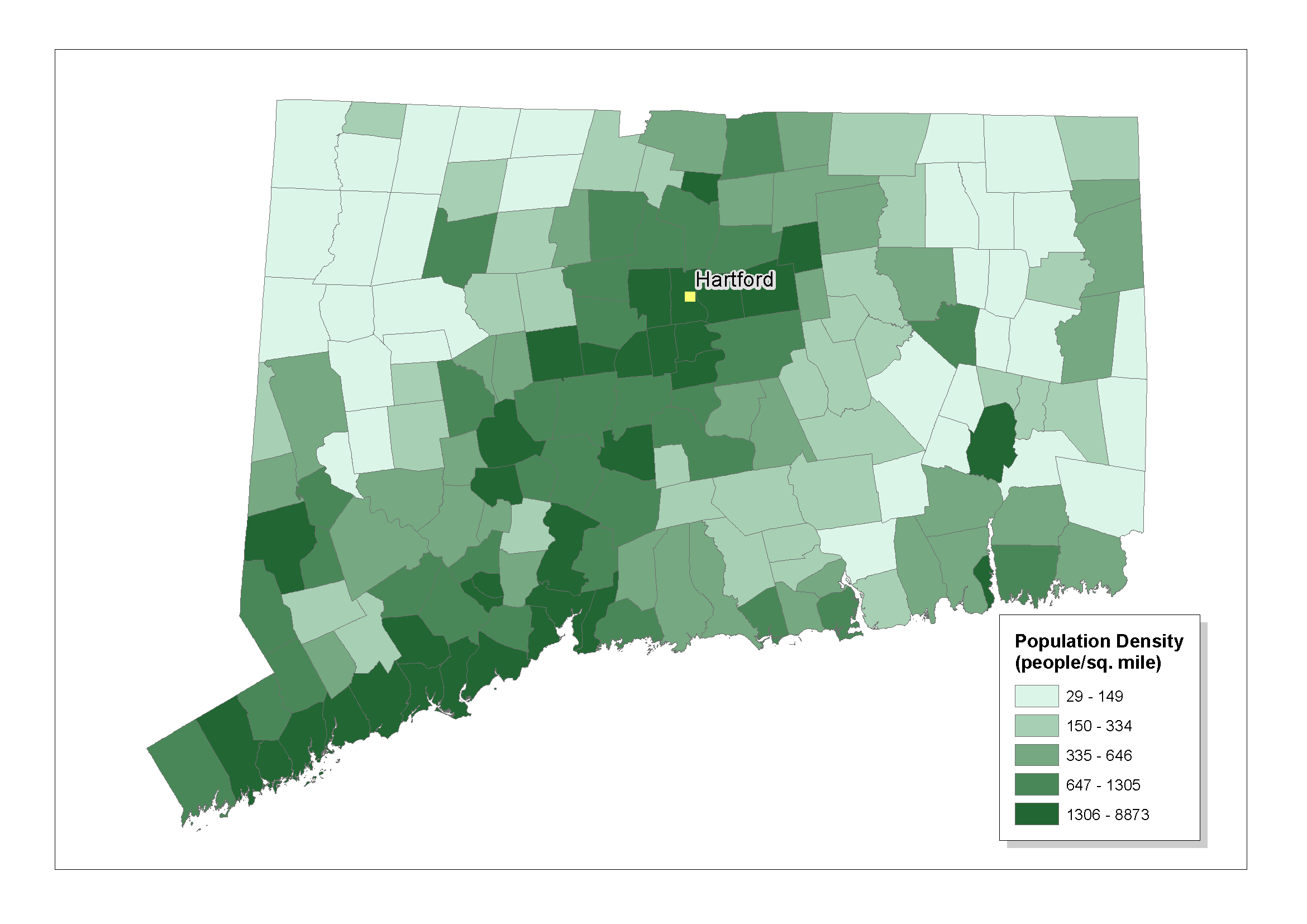
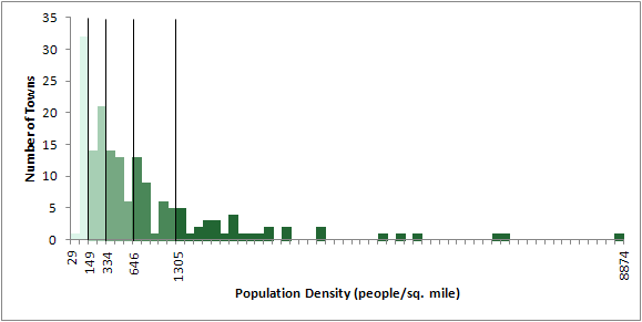
 The method is useful for mapping rectangular distributions. It is also useful for exploratory analysis, at times when you wish to develop a "feel" for the characteristics of a data distribution.

C. Arithmetic Progressions



In this method, the widths of the category intervals are increased in size at an arithmetic (that is, additive) rate. If your first category is one unit wide and you choose to increment the width one unit at a time, the second category would be two units wide, the third three units wide, and so forth to the end of the distribution.

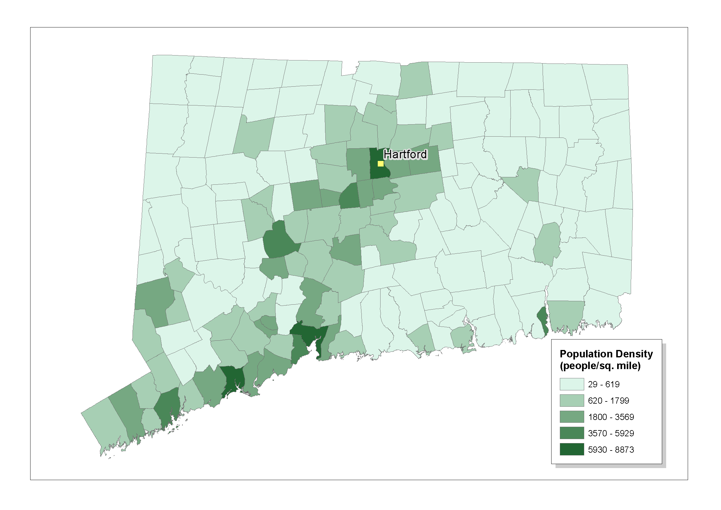
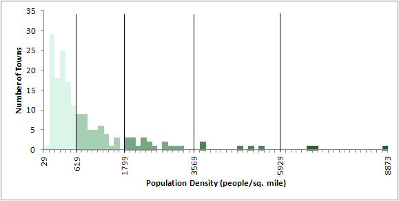
 This method can be applied effectively to data that is J-shaped with a peak at the low end of the distribution.

D. Geometric Progressions




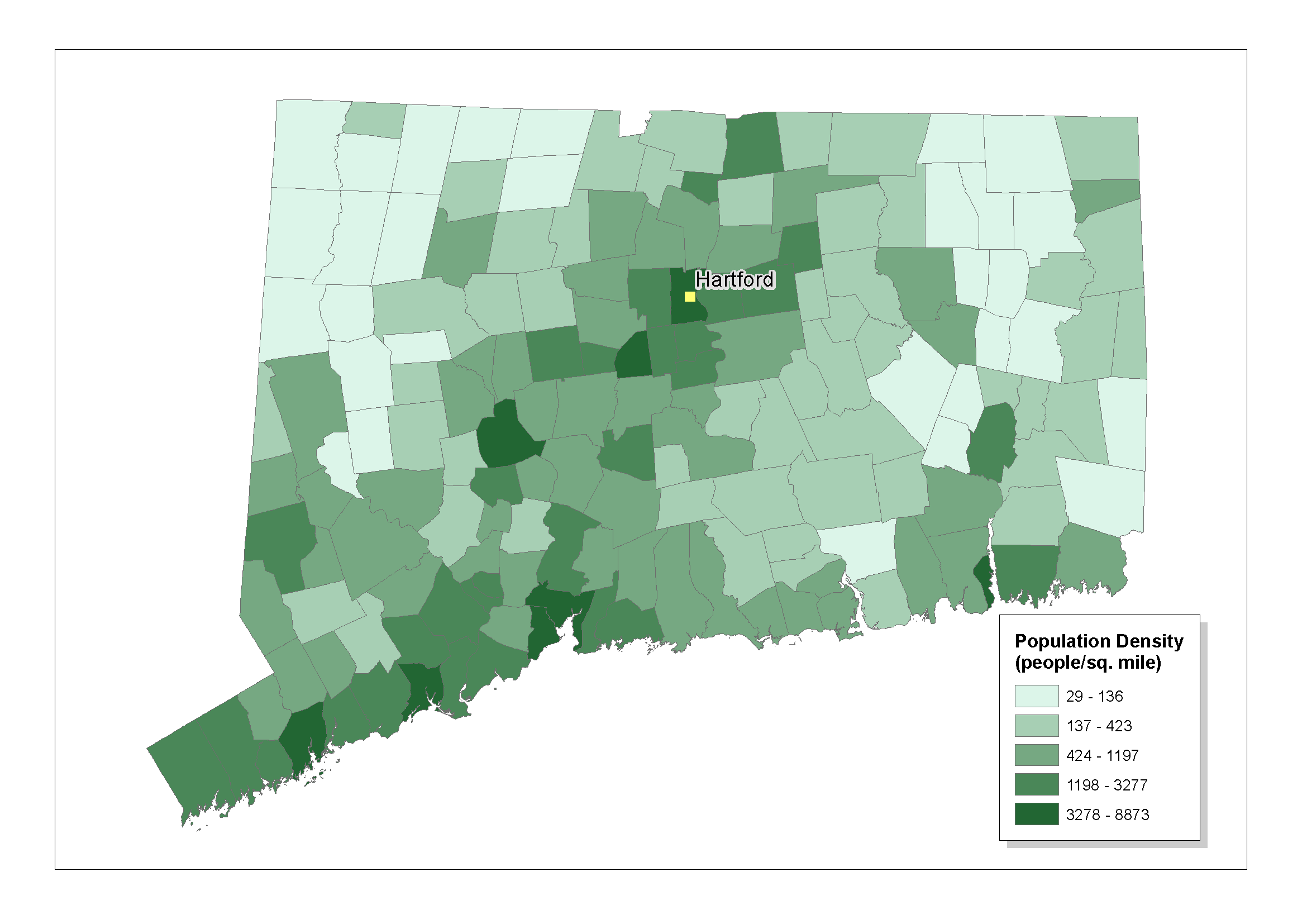
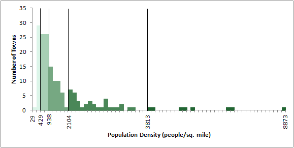
 In this method, the widths of the category intervals are increased in size at a geometric (that is, multiplicative) rate. If your first category is 2 units wide, the second would be 2x2 or 4 units wide, the third 2x2x2 or 8 units wide, and so forth to the end of the distribution.

 This method can be applied effectively to data that is J-shaped with a peak at the low end of the distribution but with a long "stretch" between low and high values.

E. Inverse Methods




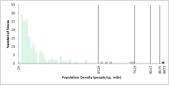
 If your data is J-shaped with a peak at the high end of the distribution, the inverses of the arithmetic and geometric progressions can be employed. By inverting the cutpoints, the smallest intervals between cutpoints will be closest together at the high end of the distribution.

F. Jenk's Method




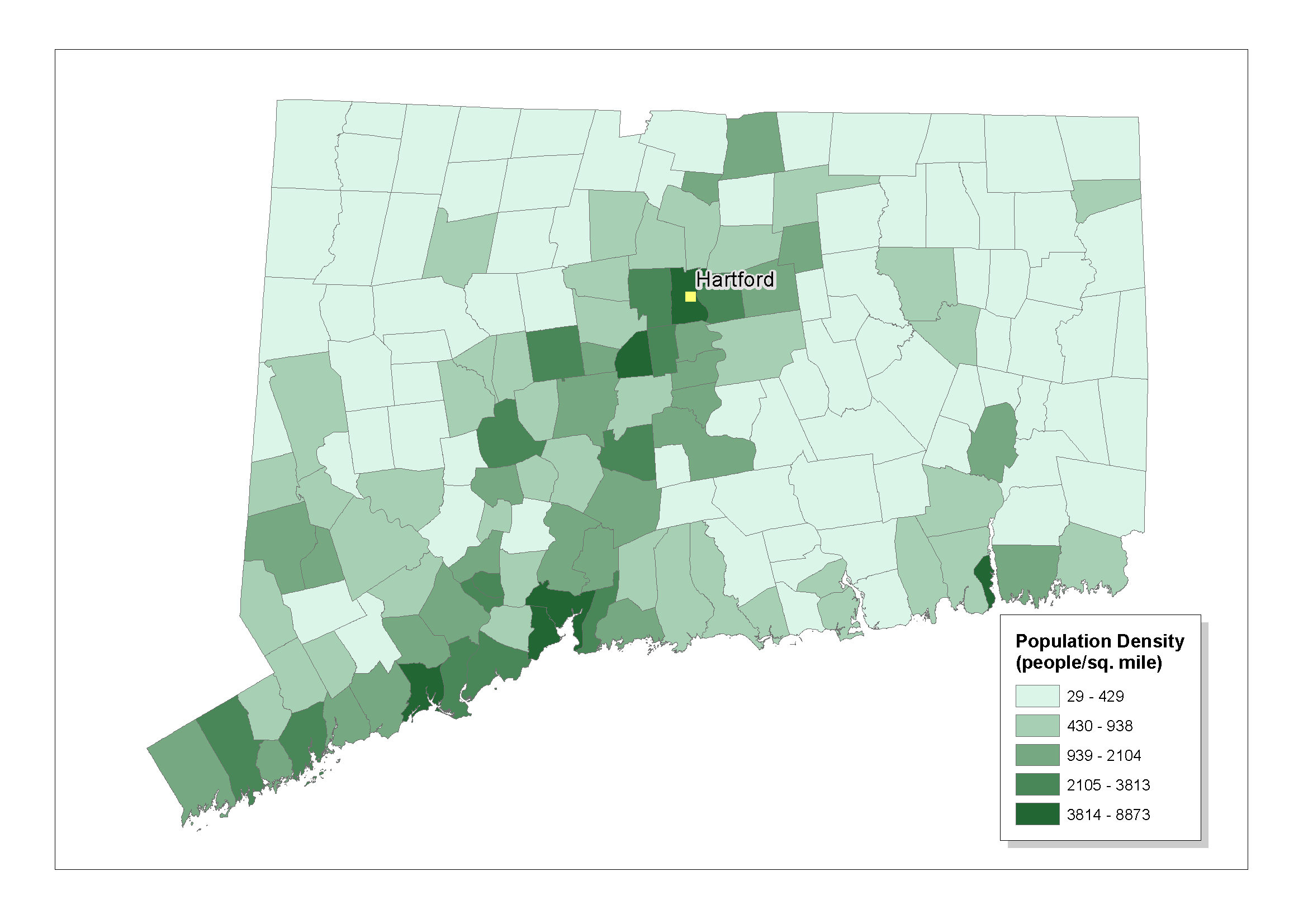
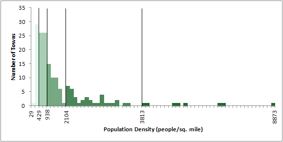
 This is a sophisticated statistical method to split the data into different classes. The categories are found by maximizing the variance between the classes and minimizing the variance within every class.

G. Standard Deviation



In this method, the standard deviation of the distribution is used to set the cutpoints above and below the average.

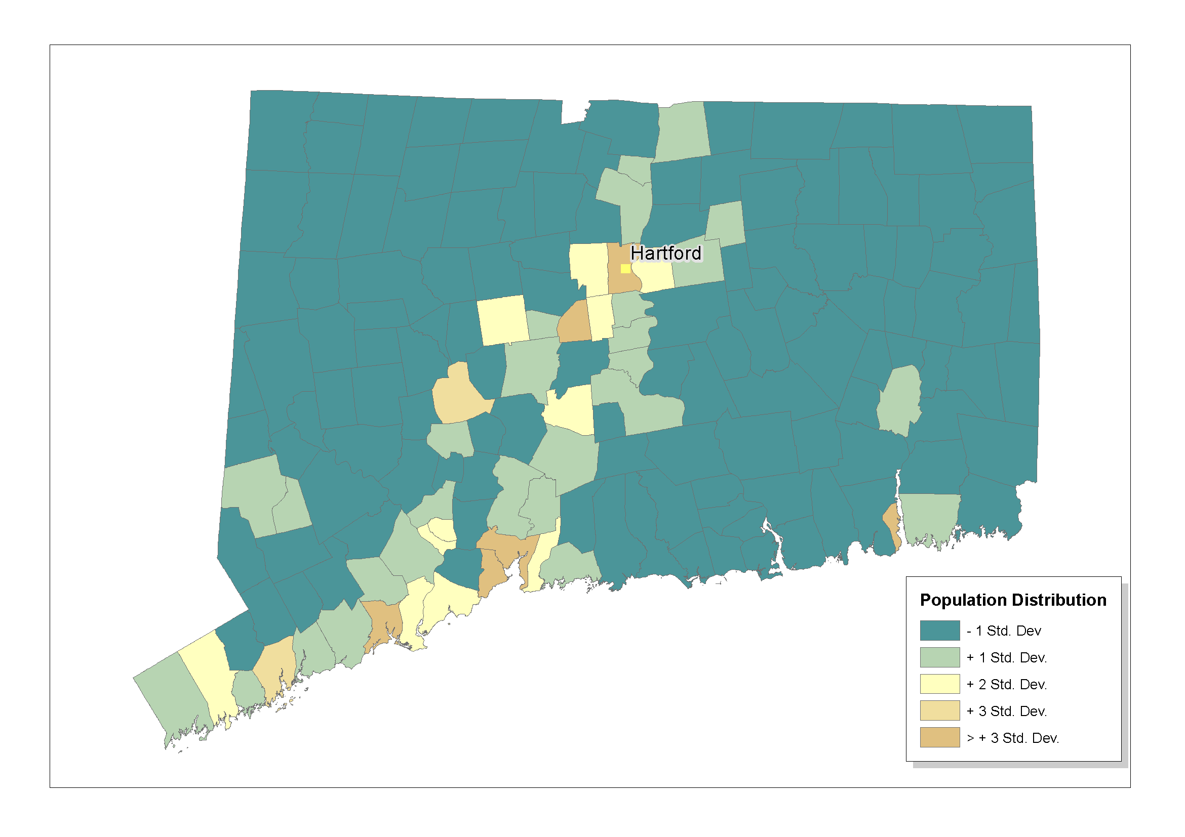
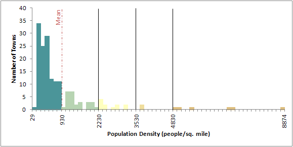
 This method can be applied to distributions that approximate a normal curve.

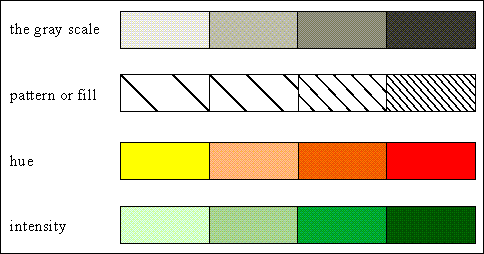
6.5 Symbolizing the Category Ranges

Once you have divided your data into categories, you must use the visual resources at your disposal to symbolize them on the map. Because your interval-ratio data have now been ordered into ordinal categories, the idea is to use color, value, or pattern to create a visual index between category symbols and their value. You can order the symbols using:


6.6 Statistical annotations are needed for some complex datasets

In some situations, you might find it useful to add statistical annotations to your map. These may indicate to the reader the nature of the statistical distribution being displayed and the means by which it was classified. Sometimes it is sufficient to note some of the descriptive statistics for a distribution, such as its range, mean, median, and mode. At other times, you may wish to add bar graphs, scattergrams, or other statistical diagrams.

---

Data Sources

Connecticut Department Of Labor. Web Address: http://www.ctdol.state.ct.us/

Minnesota Population Center. National Historical Geographic Information System: Version 2.0. Minneapolis, MN: University of Minnesota 2011. Web Address: http://www.nhgis.org/

Wolfram|Alpha online computing environment. Web address: http://www.wolframalpha.com/

Further Reading

 Coulson, Michael R.C. 1987. In the matter of class intervals for choropleth maps: With particular reference to the work of George F. Jenks. Cartographica 24 (2): 16-39.

 Evans, Ian S. 1977. The selection of class intervals. Transactions of the Institute of British Geographers New Series 2: 98-124.

 Jenks, George F. 1963. Generalization in statistical mapping. Annals of the Association of American Geographers 53: 15-26.

 Jenks, George F. and Duane S. Knos. 1961. The Use of Shading Patterns in Graded Series. Annals of the Association of American Geographers 51: 316-334.



 Go on to Problems of Realizing Ideals with Computer Systems

Return to Contents